Background

Graph-theoretic methods offer a natural and computationally efficient way of investigating communication across protein structures. There has been significant work done in this area in previous years, the majority of which has used coarse-grained residue-residue interaction networks and well-established network-theoretic methods such as shortest-pathway calculations, or the community detection method modularity.

The code underpinning this interface constructs a fully atomistic representation of the protein which encodes all interactions between atoms, covalent and non-covalent. This approach is based on the work of Meliga, Delmotte et al., Amor et al. and Song et al. [01,02,04,05,11]. The computational efficiency of our approach allows us to obtain similar information to costly non-equilibrium MD simulations, whilst our atomistic model captures information missed by coarse-grained non-energy-weighted network approaches.

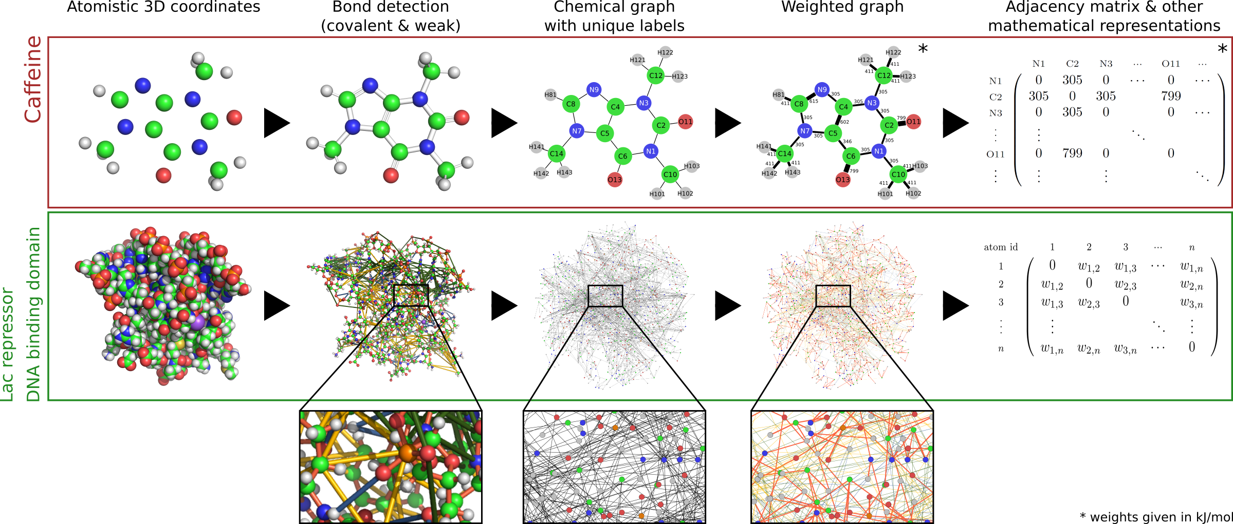
To construct the graph, all atoms in a given input structure are read in from the .pdb file and their neighbourhood is searched for potential interactions. Thus the physico-chemical properties of a biological structure are encoded in a graph, where each node represents an atom and each edge a specific interaction. Edges are weighted according to the type of interaction, differentiating between the following types:

• covalent bonds
• hydrogen bonds
• hydrophobic interactions
• salt bridges
• electrostatic interactions
• pi-pi stacking (in structures that contain DNA)

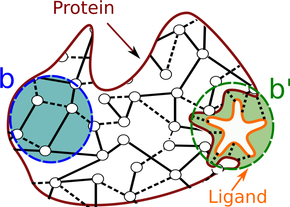
From the matrices that describe the graph constructed as above, we can derive a matrix M to extract the level of influence that the fluctuations of an edge have on any other edge in the graph (for more details see Amor et al. [02]). This level of influence is called Bond-to-bond propensity. In the context of exploring communication across protein structures, we can use propensity computations to quantify the effect of small variations of energy in one site of the biological structure (usually the active site - this is the "source site" to be selected in the Computation settings page) onto all the other bonds in the structure. This is schematically shown in Fig. 2: the graph representation of the protein includes a biologically active binding site (in green), to which a ligand is bound (in orange). We thus compute the effect of small changes in energy at the interface between the ligand and the protein structure, and quantify how much these changes impact the energy of the other bonds in the protein.

This computation results in a value of propensitynsity for each bond \(b \) in the protein. This is the raw propensity, \(\Pi^{raw}_{b}\), which reflects how closely the active site (containing the bonds \(b'\)) is coupled to each individual bond. Note that the computation includes all interactions in the protein. However, we report only the effects of the active site on the weak bonds, as it is changes in weak-bonding patterns that usually drive communication in biological structures.

To aid data analysis, we provide two extra values in the downloadable results files: the normalised propensity \(\Pi_{b}\), calculated from the raw propensity by dividing it by the sum of raw propensities across all bonds. $$ \Pi_{b} = \frac{\Pi^{raw}_{b}}{\sum_{b}\Pi^{raw}_{b}}$$ This value is then adjusted by the number of bonds in the protein, giving us a measure called adjusted propensity \(\Pi^{adj}_{b}\) for each bond in the structure. $$ \Pi^{adj}_{b} = \Pi^{b} * n_{bonds}$$ Based on the propensity value of each bond and residue we calculate a quantile score for each residue to take into account the distance effect of a graph. (More on this can be found below.) To analyse how strongly connected a site of interest for example a previously described allosteric site is, we can calculate the average residue quantile score \(\overline{p_{R,site}}\) of this site. $$\overline{p_{R,site}} = \frac{1}{N_{b,site}}\sum_{R\in site}p_{R}$$ To give an idea of how significant this site is, we sample 1000 random surrogate sites on the structure with the same size (number of residues and diameter) as the site of interest. We calculate the \(\overline{p_{R,site}}_{i}\) of each site and determine the average over this ensemble. $$\big \langle \overline{p_{R,site}} \big \rangle _{surr} = \frac{\sum_{i\in surr}\overline{p_{R,site}}_{i}}{1000}$$ This value can then be compared to the \(\overline{p_{R,site}}\) of the site of interest. To provide statistical significance we use a bootstrap with 10,000 resamples with replacement and obtain a 95% confidence interval. Details of this methodolgy can be found in Amor et al. [02].

The computation of Markov transient times is another approach to investigating communication across a given biostructure. Indeed, we can model the spread of probability across the graph that we have constructed to identify regions of the biomacromolecule that act as probability sinks, and are therefore significantly connected to the site that we have chosen as a source. A useful metaphor for this idea is the dispersion of ink on a piece of paper: if the paper was to be completely uniform, ink would diffuse as a regular circle from the point it has been dropped. Instead, we see patterns emerge following the microscopic details of the structure of the piece of paper. In the same way, modelling the spread of probability will help us individuate those regions that are reached first, dictated by the atomic organisation of the structure that we have used to construct the graph. This methodology is described in detail by Amor et al. [01], but we here provide a summary diagram.

By considering the evolution of a random walker originating on the source site, we can monitor the change in probability across all the other nodes in the structure. As the Markov time tends to infinity, the probability reaches its stationary distribution \(\pi\). Hence the speed, or number of timesteps at which each node (i.e. each atom) in the structure reaches stationarity can be used as a measure of connectivity between the source and the atom in question.

To measure such speed, we introduce the transient time \(t_{1/2}\) (thalf) which, given a set of source atoms, is the number of time steps it takes for the probability on another atom (\(i\)) to reach half its stationary value: $$t^{(i)}_{1/2} = arg_{t} min \Big[p^{(i)}_{t}\geq\frac{\pi^{(i)}}{2}\Big]$$ As such, for every atom \(i\) in the protein structure, \(t_{1/2}\) characterises the shortest random walk that connects it to the source site.

Both Bond-to-bond propensity and the calculation of Markov transient times result in distributions of values (respectively, for each bond and each atom in the structure) that are depended on the distance between the bond or atom in question and the chosen source site. To allow the analysis to consider long-range effects, we apply Quantile regression [09] to our data distributions.

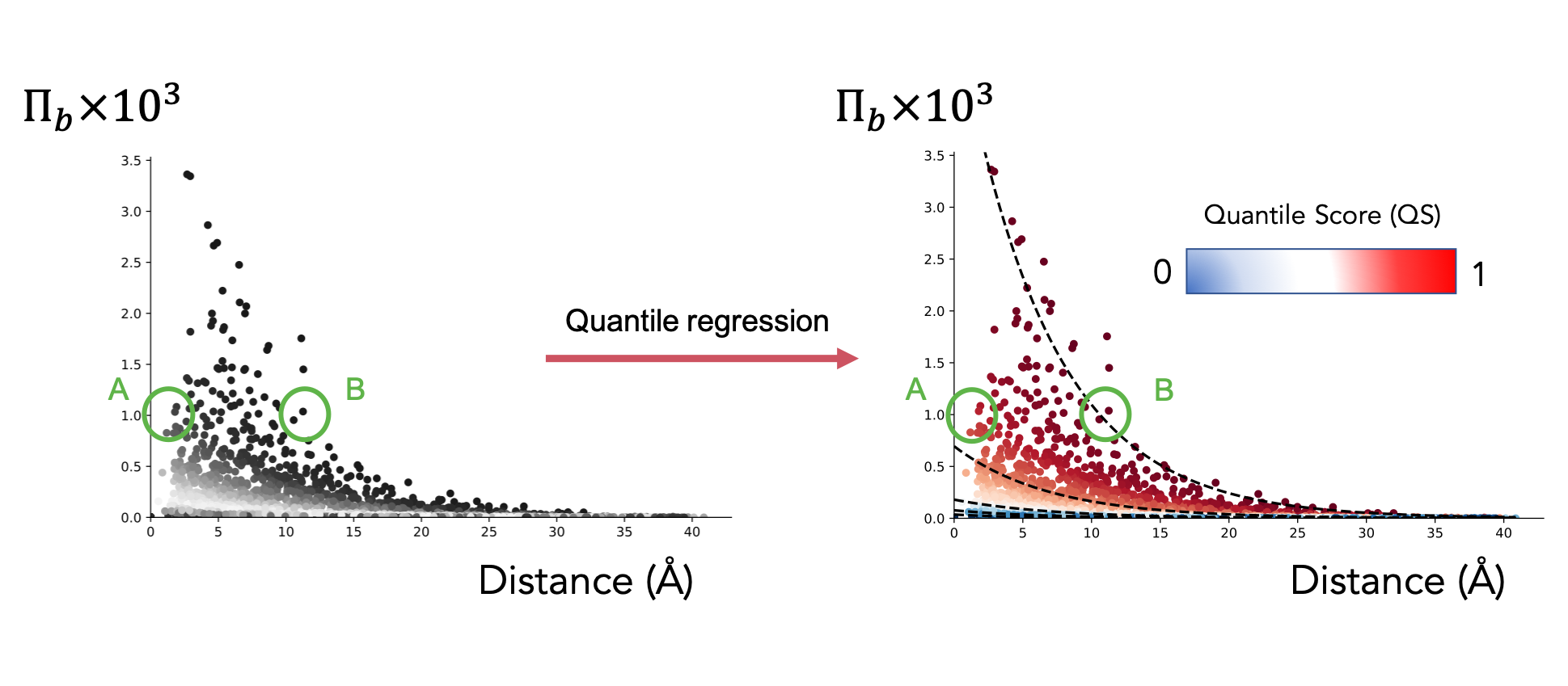
Quantile regression fits quantiles to the data distribution by solving an optimisation problem. More details can be found in Koenker et al. [09]. The quantile scores (values between 0 and 1 assigned to every bond depending on the quantile the bond lies on) help us avoid distance bias in our analysis. For example, two bonds A and B with equal propensity (as shown in the figure) would seem connected to the source site with equal intensity. However, bond B is at a greater distance from said source than bond A. Quantile regression therefore assigns a higher score to bond B to reflect its more significant role.

Similarly, we compare the result distribution of each structure to a database of Bond-to-bond propensity and Markov transient results, to assess the communication within the input structure with respect to a benchmark set of proteins with different shapes. This benchmark set consists of 100 proteins taken from the SCOP database [10] and is discussed in more detail by Amor et al. [02]. This second quantile regression yields the test set quantile score, a value for each bond (in Bond-to-bond propensity computations) and each atom (in Markov transient computations) which expresses (as a 0 to 1 value) the strength (or speed) of communication with the active site compared to all other bonds (or nodes) in the selected structure and in the 100 structures in the benchmark set.